The basic flow of the probability pages goes like this:
- Definitions
- Set operations
- Probability axioms
- Counting: Permutations & combinations
- Conditional probability
- Independence of events
- Bayesian probability (this page)
Bayes' theorem
Linking conditional probabilities
Bayes' theorem is a way of relating conditional probabilities like P(A|B) and P(B|A). It is extremely useful not only for solving difficult-to-solve problems, but also in lending a lot of insight into how probability-driven phenomena work. Let's derive it first, then do some work with it.
Recall that for sets A and B (outcomes of a probability experiment) we can write two conditional probabilities:
$$ \begin{align} P(A|B) &= \frac{P(A \cap B)}{P(B)}, \; \text{and} \\[5pt] P(B|A) &= \frac{P(A \cap B)}{P(A)}. \end{align}$$
Recall that there is no preferred order in finding intersections of sets, so $(A \cap B) = (B \cap A).$
Now we can solve each of the equations above for $A \cap B$ like this:
$$ \begin{align} P(A \cap B) &= P(A|B)P(B), \; \text{and} \\[5pt] P(A \cap B) &= P(B|A)P(A) \end{align}$$
Now we can link these equations together, eliminating $P(A \cap B)$:
$$P(A|B)P(B) = P(B|A)P(A)$$
Finally, dividing by P(B) on both sides gives
$$P(A|B) = \frac{P(B|A)P(A)}{P(B)},$$
which is Baye's rule. Notice how it provides a link between the conditional probabilities P(A|B) and P(B|A).
Example 1
Suppose that on average, 1% of all people have a certain disease. A test for the disease has a 95% rate of detection. The test also has a 5% false-positive rate. Calculate the probability that a person who gets a positive test actually has the disease.
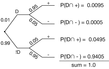
That looks about right. For people who have the disease, the probability of getting a positive test is 95%, thus the probability of getting a negative test (the only other option) is 5%, and so on. We assume that getting the disease and testing for it are independent events, thus we can calculate the probabilities of all of the intersections, as shown.
What we're being asked to find is P(D|+), the probability that if a positive test result is given, that the person will actually have the disease. Here's where we use Bayes' rule:
$$P(A|B) = \frac{P(B|A)P(A)}{P(B)}$$
Adapting it to our problem, we get
$$P(D|+) = \frac{P(+|D)P(D)}{P(+)}$$
We just have to fill in the numbers. We know, from the setup information, that P(+|D) = 0.95, and we know that P(D) = 0.01, so that takes care of the numerator.
For the denominator, we need the total probability of a + test. That's just the sum of the disjoint intersections $\{D \cap +\}$ and $\{!D \cap +\}.$
$$ \begin{align} P(+) &= P(D \cap +) + P(!D \cap +) \\[5pt] &= 0.0095 + 0.0495 \\[5pt] &= 0.059 \end{align}$$
So finally, we have
$$ \begin{align} P(D|+) &= \frac{P(+|D)P(D)}{P(+)} \\[5pt] &= \frac{0.95(0.01)}{0.059} \\[5pt] &= 16.1 \% \end{align}$$
Now that seems pretty small, given that the test is 95% accurate at detecting disease. The hitch is that the prevalence of the disease is so small; just 1% of people have it. Let's see if our answer makes any sense graphically. Here is a sampling of 100 people (dots). The red dot is our one person (on average) with the disease.

The white dots are our 5% false positives. So, roughly speaking, the chance of a person getting a positive test and actually having the disease is about 1 out of those six people, 1/6, or 16.7%, so that's about right. Our calculation just cleaned up around the edges of this approximation. For example, once we remove our one disease carrier from the mix, those five false positives are against a background of 99 people, not 100.
Here is a graph of P(D|+) vs. the probability of having the disease, P(D). Notice that as the prevalence of the disease increases, the chance that a positive test is a real diagnosis increases. If the prevalence (the number of people in the population who, on average, have the disease) reaches 20%, then our positive tests would mean more than an 80% chance of actually having it.

Bayesian analysis like this is a powerful tool for managing our expectations in many situations such as this test. We'll work through more examples below.
Bayesian inference
Modifying our expectations with new data
Let's refer to the first example above and ask this important question: What if we took a second drug test and it, too, turned out positive? What then would be the probability of actually having the disease? That is, we're trying to find P(D|++), where "++" means a positive test result twice in a row.
There are a number of ways of calculating this probabilty using Bayes' rule. We could make a modified tree:
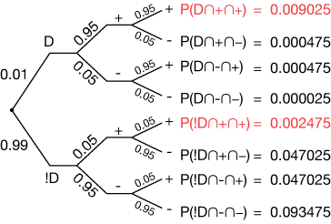
where the probabilities in red are they ones we'll need in the calculation. Our Bayes' rule expression will look like this:
$$P(D|++) = \frac{P(++|D)P(D)}{P(++)}$$
Now notice that this is really just the same as the expression we used in the first example, just with " + " replaced by " ++ ". P(D) is the same, and P(++|D) is just 0.952 = 0.0925. The denominator can be expanded like this:
$$ \begin{align} P(++) &= P((D \cap +) \cap +) + P((!D \cap +) \cap +) \\[5pt] &= 0.01(0.95)(0.95) + 0.99(0.05)(0.05) \\[5pt] &= 0.009025 + 0.002475 \\[5pt] &= 0.0115 \end{align}$$
Now we can find P(D|++):
$$ \begin{align} P(D|++) &= \frac{P(++|D)P(D)}{P(++)} \\[5pt] &= \frac{0.9025(0.01)}{0.0115} \\[5pt] &= 78.5 \% \end{align}$$
That's quite an improvement, and it suggests that this test might not be so bad, as long as we're willing and able to do a second test after a positive result.
As an exercise, verify for yourself that adding a third positive test increases the chance of having the disease to 98.6%.
Bayesian spam filtering
Spam emails are unwanted or unsolicited emails sent by a party either trying to sell you something or otherwise get money or valuable information. Email servers and software try to limit the number of known spam emails that actually get to the end user, or at least to gather them in a holding place until the user can judge for herself whether they're real.
Bayesian inference is sometimes used in spam filtering. It works like this: Each email is parsed (read) and key words and phrases are collected. These are compared to databases of spam and non-spam emails, yielding a probability that an email is spam. If we let W stand for "words" and S stand for "spam," then we have P(W) = the probability that certain words occur, and P(S) = the probability that an email is spam. We can write a Bayes' rule expression like this:
$$P(S|W) = \frac{P(W|S)P(S)}{P(W)}$$
The conditional probability P(S|W) is the probability that if an email contains certain words, it will be a spam. We can link it to P(W|S) through Bayes' rule.
The probability that a spam will contain certain key words and phrases is relatively easy to measure just by parsing millions of emails and looking for them.
Likewise, it's relatively easy to create a database and calculate a probability of finding those key words and phrases in any email, giving us P(W).
In this way, software and mail servers can generate a probability that any given email is spam, and the user can set a threshold of what she views and what she discards.
Of course, there are ways to get around this, and people with nefarious intentions generally find them. But it's a start. One clever, but probably time consuming way of getting around such a Bayesian filter is to spell out a message in images, like this:

A weather example
Let's say you are planning an outdoor activity. You look outside in the morning and the sky is cloudy. Should you cancel? You know these facts:
- 60% of all rainy days in your area start out cloudy.
- About 50% of all days in your area start out cloudy.
- At this time of year, you only get about four days of rain per month. That's 4/30 or 13.3% of the days.
Given all that, what is the chance of rain today. That is, calculate P(R|C), where R stands for rain and C stands for clouds in the morning.
The Bayes' rule expression is
$$P(R|C) = \frac{P(C|R)P(R)}{P(C)}$$
In the numerator, P(C|R) is the probability that when it rains, it's cloudy in the morning. That's our 60%, or P(C|R) = 0.60. We also have the probability of rain, P(R) = 0.133. Finally, the probability of clouds is given: P(C) = 0.4.
So our probability of rain today is
$$ \begin{align} P(R|C) &= \frac{P(C|R)P(R)}{P(C)} \\[5pt] &= \frac{0.6(0.133)}{0.4} \\[5pt] &\approx 20\% \end{align}$$
That's too low a probability to cancel. Put yourself in a position to succeed!
Example – Jars of marbles
Let's say we have two jars, call them J1 and J2, each containing six marbles. J1 contains 3 blue (B) and 3 red (R) marbles, and J2 contains 4 B and 2 R. Calculate the probability that if one marble is drawn in the blind from a randomly-chosen jar, that jar will be J1.


The Probability is
$$P(J_1|B) = \frac{P(B|J_1)P(J_1)}{P(B)}$$
We know that P(B|J1) is ½. We know that there is a 50-50 chance of choosing each jar, so P(J1) = ½. For the denominator, we have
$$ \begin{align} P(B) &= P(B \cap J_1) + P(B \cap J_1) \\[5pt] &= \frac{1}{4} + \frac{1}{3} = \frac{7}{12} \end{align}$$
Now the probability we're looking for is
$$P(J_1|B) = \frac{\frac{1}{2} \frac{1}{2}}{\frac{7}{12}} = \frac{3}{7}$$
See if you can calculate P(J2|B) in a similar way. The result should be 2/7.
Practice problems
-
A doctor visits a sick child. She knows that in the neighborhood at the moment, 90% of the sick children have the flue and the other 10% have the measles. Assume that in this neighborhood at this time, there are no other illnesses circulating. Let F be a case of the flu and M be measles.
One sign of measles is a rash (R). Assume that the probability of having a rash if one has measles is P(R|M) = 0.95. Sometimes kids with the flue develop a rash, with probability P(R|F) = 0.075.
Upon examining the child, the doctor finds a rash. Calculate the probability that the child as measles.
Solution
We know that
$$ \begin{align} P(R|F) &= 0.075 \\[5pt] P(R|M) &= 0.95 \\[5pt] P(F) &= 0.9 \\[5pt] P(M) &= 0.1 \end{align}$$
The probability that a rash predicts the flu is
$$P(F|R) = \frac{P{R|F)P(F)}}{P(R)}$$
The numerator is straightforward: 0.75(0.9). The expanded denominator is
$$P(R) = P(R \cap F) + P(R \cap M),$$
but we don't know those straight off. We can calculate them, however, using the definition of conditional probability. For the first term, we know that
$$P(R|F) = \frac{P(R \cap F)}{P(F)}.$$
Now solving for $P(R \cap F)$ gives:
$$P(R \cap F) = P(R|F)P(F).$$
Likewise, we have
$$P(R \cap M) = P(R|M)P(M).$$
So our denominator is
$$ \begin{align} &P(R \cap F) + P(R \cap M) \\[5pt] &= P(R|F)P(F) + P(R|M)P(M) \\[5pt] &= 0.075(0.9) + 0.1(0.95) \\[5pt] &= 0.1625 \end{align}$$
Finally, our probability is
$$P(F|R) = \frac{0.075(0.9)}{0.1625} \approx 42\%$$
While measles has a higher chance of producing a rash, the prevalance of the flu in this population is much higher.
-
A group of physicians were asked what the chance of breast cancer would be in a woman who was originally thought to have a 1% risk of cancer, but who ended up with a positive mammogram result. Mammograms typically accurately identify about 80% of cancerous tumors and 90% of benign (non-cancerous) tumors. 95% of the physicians estimated the probability of cancer to be about 75%. Were they correct?
Solution
Let's call cancer C, and not sick !C. We'll use + and - for the test results. Here is a tree diagram of this scenario:

We want to calculate
$$P(C|+) = \frac{P(+|C)P(C)}{P(+)}$$
Expanding the denominator gives
$$P(+ \cap C) + P(+ \cap !C) = 0.008 + 0.099$$
So our probability is
$$ \begin{align} P(C|+) &= \frac{0.8(0.01)}{0.008 + 0.099} \\[5pt] &= 7.4 \% \end{align}$$
So the doctors were high in their estimate by about a factor of ten.
-
Two manufacturing assembly lines produce the same product. Line A produces 1,000 parts per week, of which 100 are defective. Line B produces 2,000 parts per week, of which 75 are defective. If you choose a part randomly from the combined output of both lines, what is the probability that it is defective? If it is defective, what is the probability that it was produced by line A?
Solution
We'll let A stand for "manufactured on line A" and B stand for "manufactured on line B." Let D stand for "defective." Here are the probabilities we know:
$$ \begin{align} P(A) &= \frac{1}{3} \\[5pt] P(B) &= \frac{2}{3} \\[5pt] P(D|A) &= \frac{100}{1000} = 0.1 \\[5pt] P(D|B) &= \frac{75}{2000} = 0.0375 \end{align}$$
The total probability that a part will be defective is
$$P(D \cap A) + P(D \cap B),$$
which we get this way:
$$ \begin{align} &P(A)P(D|A) + P(B)P(D|B) \\[5pt] &= \frac{1}{3}(0.1) + \frac{2}{3}(0.0375) \\[5pt] &= 0.025 \end{align}$$
That's also the denominator of our Bayes' rule expression,
$$P(A|D) = \frac{P(D|A)P(A)}{P(D)}$$
So our probability is
$$\frac{0.1(0.333)}{0.025} = 57 \%$$
Axiom
An axiom is a statement that is self-evidently true, accepted or long-established, but which can't necessarily be proven so. A famous axiom is Euclid's first postulate, also known as the transitive property: "Things that are equal to the same thing are equal to each other," or If a = b and c = b, then a = c.
Induction
When we reason inductively, or use induction to reason, we extend a pattern. The sun has risen every day of my life, so I'm reasonably confident it will rise again tomorrow. That's induction. To extend a series like 2, 4, 6, 8, x, by concluding that x = 10 is also induction.
Axiom
An axiom is a statement that is regarded as being true or established, or self-evidently true. Axioms cannot be proven.
A fundamental axiom is the transcendental property: Things that are equal to the same thing are equal to each other, or if a = b and c = b, then a = c.
Theorem
A theorem is a general proposition in mathematics or other forms of reasoning that may not be self-evident, but can be proved by a chain of reasoning based on things that are already known to be true.

![]()
xaktly.com by Dr. Jeff Cruzan is licensed under a Creative Commons Attribution-NonCommercial-ShareAlike 3.0 Unported License. © 2012-2025, Jeff Cruzan. All text and images on this website not specifically attributed to another source were created by me and I reserve all rights as to their use. Any opinions expressed on this website are entirely mine, and do not necessarily reflect the views of any of my employers. Please feel free to send any questions or comments to jeff.cruzan@verizon.net.