The basic flow of the probability pages goes like this:
- Definitions (this page)
- Set operations
- Probability axioms
- Counting: Permutations & combinations
- Conditional probability
- Independence of events
- Bayesian probability
Speaking the language of probability
More things in the universe are governed completely by random action than you might realize. Yet everything still works. We describe that randomness using the language, axioms and theorems of probability. To study probability is to study
- chance
- variation
- error
- likelihood
- risk
- odds, and so on.
To get started learning about probability, we first need to learn to speak a common language. In this section we'll take care of the basic definitions of terms we'll use frequently.
In the following section, Probability Axioms, we'll learn about what we can do with those defined things using just a few axioms (rules we can't necessarily prove, but we all agree are true). From those we'll develop all of the other rules and theorems we'll need to study probability.
Things that are governed strictly by random chance and the laws of probability are said to be stochastic.
Probability experiments & outcomes
In probability theory, an experiment is something that we can do repeatedly and that can have more than one possible outcome (with only one outcome, we don't need probability, right?). We can list all possible outcomes, and we generally do so in set notation, such as {a, b, c}, using curly braces.
In fact, sets, set notation and the manipulation of sets will be a key feature of our exploration of probability.
For any probability experiment, we'll want to build a model that predicts the probability of any given outcome. We'll do that by building up our knowledge from simple to more complex experiments.
| Experiment | Outcomes |
|---|---|
| Flipping a coin | {H, T} |
| Tossing a tetrahedral (four-sided) die |
{1, 2, 4, 5} |
| Tossing a six-sided die | {1, 2, 3, 4, 5, 6} |
| Tossing a six-sided die twice, take the sum |
{2, 3, 4, 5, 6, 7, 8, 9, 10, 11, 12} |
| Drawing a playing card | {52 possibilities} |
Sample spaces
The sample space of a probability experiment is the set containing all possible outcomes. We often label the sample space, with the (capital) Greek letter omega (Ω). We'll use basic set notation like Ω = {H, T} for flipping a coin (H = heads, T = tails). It's also nice once in a while to use a box diagram like the one shown below. It's just a box listing all of the possible outcomes, and labeled Ω.

Image: U.S. Mint Catalog

Here are representations of the sample space for tossing a single tetrahedral (four-sided) die. (When such a die is tossed, one number shows on three sides at the peak of the pyramid.)
![]()

A tetrahedral die. "Die" is the singular of "dice."
Here are representations of the sample space for the experiment of throwing two six-sided dice at the same time, with possible outcomes being the sum of the numbers on the dice.


Requirements of the sample space
In order to be able to do anything meaningful with a probability experiment and its sample space, we need it to have two important properties
- The outcomes must be mutually exclusive. For example, if a coin toss comes up heads, then it can't possibly also come up tails. If six-sided die lands with four up, then 1, 2, 3, 5 and 6 are ruled out or excluded.
- The outcomes must be collectively exhaustive. That is, all possible outcomes of the experiment must be listed in the set. The set S = {1, 2, 3, 4, 5} is not a complete list of the outcomes of throwing a single six-sided die because 6 is missing.
The sample space of a probability experiment must be
- mutually exclusive
- collectively exhaustive.
Probability notation
For each outcome in a sample space, we'll want to assign a probability value: what is the likelihood that outcome x will occur if the experiment is run once? Let's take a coin flip as our example. The sample set is Ω = {H, T}. We'll call the probability that the coin comes up heads P(H) and the probability that it comes up tails P(T).
Notice that the two outcomes are mutually exclusive, so the probability of the coin landing with tails up is the same as the probability that it does not land with heads up. We can write this situation like this:
$$P(T) = P(!H),$$
The probability P(!H) can be read as "the probability of not tossing heads," where the exclamation point means and is pronounced "not." It is called the compliment of P(H), and can also be written as P(HC).
P(H) |
Probability of tossing heads |
P(T) |
Probability of tossing tails |
P(!H) or P(HC) |
Probability of not tossing heads P(!H) = P(T) |
P(!T) or P(TC) |
Probability of not tossing tails P(!T) = P(H) |
In the coin experiment, where there are only two possible outcomes, we could also just use P(H) and P(!H) to specify the probabilities of all possible outcomes.
Probabilities
The probability that an even or outcome of probability experiment occurs is $P(x_i),$ where x is the ith outcome.
The sum of the probabilities of each possible outcome in the sample space containing n discrete outcomes is 1
$$\sum_{i=1}^n P(x_i) = 1$$
The probability of an event is always between 0 and 1: $0 \le P(x_i) \le 1.$
Appropriateness of sample spaces
This is a bit of an absurd example, but it will illustrate a worthwhile point: we need to pare our sample set down to observations that are relevant.
Consider the experiment of flipping a coin, with outcomes heads (H) or tails (T). Now let's consider flipping a coin while watching the cat. Sometimes the coin comes up heads while the cat is in the room and sometimes it's tails. Sometimes the cat isn't in the room when either H or T occur. Our possibilities are:

We've used our new "not" notation here to signify that the cat is either in the room or it isn't.
Now is this an appropriate set of possible outcomes? Well, maybe, if you're genuinely concerned about doing measurements to see if the presence of the cat has anything to do with flipping coins. But in general, that seems kind of silly, and we'd probably agree that inclusion of the cat isn't going to change our expectation that the probabilies of a fairly-flipped coin coming up heads or tails are the same (they are both ½ or 50%).
The point is that we really ought to look for sample spaces that are as simple as possible to fairly represent the experiment being done.
Tree diagrams
Sometimes a tree diagram is very useful for mapping out all of the possible outcomes of a probability experiment. Here is a tree diagram showing all possibilities of rolling a tetrahedral (four-sided) die twice — or rolling two dice that can be distinguished from one another, say one blue one and one red one.
For the first roll, there are four possibilities, the set $\Omega = \{1, 2, 3, 4\}.$ Each of those has an additional four possibilities for the second roll, giving the complete set of 16 possibilities:
$$ \Omega = \begin{Bmatrix} 11, & 12, & 13, & 14, \\ 21, & 22, & 23, & 24, \\ 31, & 32, & 33, & 34, \\ 41, & 42, & 43, & 44, \end{Bmatrix}$$
Obviously, to add any more rolls to this tree would make it complicated and difficult to draw, but drawing a simple tree can often help us to establish a pattern and guess the rest by inductive reasoning. It's easy to see, for example, that adding another roll would bring the number of possibilities to 64. We'll use trees like this a lot in examples in other sections.

Example 1
What is the probability of drawing a number card (2, 3, ..., 9, 10) from a standard deck of 52 playing cards?
We can simplify the sample space a little bit here by just considering one of the four possible suits of cards. It looks like this:

There are 14 different cards in each suit, three of which are face cards, and one is an ace (which we could call a 1, but I'll keep it separate from the number cards here).
The green box highlights the number cards. There are ten of them, so our probability of selecting one in the blind is
$$P(number) = \frac{10}{14} = \frac{5}{7},$$
or just over 71%. Let's just check to make sure our initial approximation of using just one suit is OK. We'd have four times the number of number cards, but also four times the number of total cards if we counted the whole deck, so those fractions above would be multiplied by $\frac{4}{4},$ which is one, so we're OK.
Example 2
A fair coin is tossed three times. Calculate the probabilities that
- At least one head (H) is obtained
- Exactly one head is obtained
The easiest way to find these probabilities is to sketch a tree diagram like this one.

Now we can easily see that in this sample space (Ω), there are eight possible outcomes. Another way to sketch it is like this:

From any of these representations, it's easy to see that seven of eight have at least one H, and only one has exactly one H. So our probabilities are
$$ \begin{align} P(\text{at least one H}) &= \frac{7}{8} \\[5pt] P(\text{only one H}) &= \frac{1}{8} \end{align}$$
Now there's one thing we should bear in mind: These tree diagrams aren't always so simple. For example, consider the possibilities for five flips of a coin. Would you really want to write that all out? We'll have to find better ways of counting outcomes, and we will.
Example 3
Let's invent a new dice game. Each of two players gets one roll of a single die. If the highest of the two dice is 4 or below, player 1 wins. If the highest roll is 5 or 6, then player 2 wins. Each player can bet on the outcome in advance of the rolls. Who is likelier to win, player 1 or player 2?
Here's a table of all possible outcomes for two rolls:

It might be tempting to assume that because there are four possibilities for each roll for player 1 to win, and only two for player 2, that player 1 has the best bet. But a look at the sample space shows 4 × 4 = 16 possibilities for player 1 to win and 20 possibilites (magenta region) for a player 2 win.
The probability of winning for each player is
$$ \begin{align} P(1) &= \frac{16}{36} = \frac{4}{9} \\[5pt] P(2) &= \frac{20}{36} = \frac{5}{9} \end{align}$$
Notice that the sum of these probabilities, that is, the probability that either player 1 or player 2 wins is
$$\frac{4}{9} + \frac{5}{9} = \frac{9}{9} = 1,$$
which is to say that someone has to win. In other words, the sample space is exhaustive. The
Sample spaces: discrete vs. continuous
There are two kinds of probability sample spaces, discrete and continuous. Let's illustrate them with examples.
Discrete sample spaces
Consider making two rolls with a tetrahedral die (or equivalently one roll of two equivalent but distinguishable dice at the same time). Here is a table of the possible outcomes:

For this experiment, there are a finite number of possible outcomes. That number is either 16 or 10, depending on whether the order of the numbers matters. That is, is the outcome (1, 2) different than (2, 1)? That will depend on how the experiment is defined.
What's important in this context is that the number of possible outcomes is finite, and the set defined by the grid is exhastive (includes all possible outcomes). Now let's compare that to a continuous probability example.
Continuous sample spaces
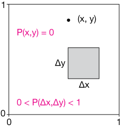
Think about a dart board of sorts that is 1 meter on a side (1 m × 1 m). Imagine we throw darts at the board (and that we're incapable of missing it altogether). Each dart will have a real-number set of (x, y) coordinates to mark its position on the board. Now this experiment has an infinitely large set of possible outcomes.

This is an example of continous probability. The number of possible outcomes is not countable as in the discrete example – it's infinite ("discrete," by the way, means countable).
One interesting consequence of this sample space is that the probability, P(x, y) of hitting any one location (x, y) with our dart is actually zero. That's because we can't actually specify, to any given precision, a point in that space. You could try to specify one, but I could always insist on some more digits of precision.
What we can do in this case, is to calculate the probability of hitting the board in a particular zone, say the upper left quarter. As long as we do that, we can have finite, non-zero probabilities.
Venn diagrams and set operations
Venn diagrams can be very useful for visualizing what's going on as we combine and manipulate probability sets. We'll start with a rectangle to represent our whole probability sample space, Ω.

Within that space, we can specify some subsets, like A and B below. Subset A might be all of the ways of rolling a sum of seven with two cubic dice, and B might all possible ways of rolling a sum of six, just as an example. They are both fully contained within the universe (Ω) of possible two-die rolls, but they are mutually exclusive: Either a seven is rolled or a six, but the two sets can't overlap. We say that the intersection of the two, $A \cap B,$ is the empty set, { } or ∅.

In the case above, sets A and B are said to be disjoint because they have no elements in common.
Now let's imagine that A is the set of ways to roll a total of seven with two cubic dice, and B is the set of rolls containing at least one 2. These sets can overlap because we can roll a 5-2 or a 2-5. That overlap is given by the intersection of sets A and B, $A \cap B = \{52, 25\}.$ The Venn diagram is shown below.

Now suppose that we'd like to roll two cubic dice and find the probability of rolling either a total of seven or obtaining at least one two. For that we use the union of sets A and B, $A \cup B,$ which is the two sets combined. An outcome from either will fit our needs. As we'll note later, sometimes we need to be careful with unions because we might accidentally count the intersection twice when we don't want to. More on that later.

Finally, we might want to know the probability of our result not being in set A. For example, we might want to know the probability of rolling two cubic dice and having the result not add up to 7. That probability is $P(!A),$ and the set is $!A,$ which is read "not A." An alternative is to use the notation AC, which means "the complement of A," or everything not in set A. In the Venn diagram below, the blue area is everything not in set A.

In quite a few cases, calculating a probability of an event is difficult, but calculating the probability of the event not happening (its complement) is easier, and that's really the best way to solve the problem.
Practice problems
| 1. |
Write the sample space for these probability experiments:
Solutions(a) dice: The sample set is $$ \Omega = \begin{Bmatrix} 11, & 12, & 13, & 14, \\ 21, & 22, & 23, & 24, \\ 31, & 32, & 33, & 34, \\ 41, & 42, & 43, & 44, \\ 51, & 52, & 53, & 54, \\ 61, & 62, & 63, & 64, \\ \end{Bmatrix}$$ where the first number is what shows up on the six-sided die and the second is from the tetrahedral die. (b) dial The sample set for the dial is $$\Omega = \{A, B, C, D, E, F, G, H, I, J\}$$ (c) cards Here's a picture of the sample space for the black cards:
(d) Coin + spinner: The sample set is $$ \Omega = \begin{Bmatrix} HA,HB,HC,HD,HE,\\ HF,HG,HH,HI,HJ,\\ TA,TB,TC,TD,TE,\\ TF,TG,TH,TI,TJ,\\ \end{Bmatrix}$$ |
| 2. |
Consider the probability outcome of the sum of the values showing on two six-sided dice. Write the sample space for this set, then calculate the probabilities for sums of 2 - 12. SolutionHere's one way to represent the sample space, the number pairs are first-die, second-die. The diagonals represent rolls with the same dice totals, and the red numbers are the frequencies of those totals. For example, there is only one way to arrive at a sum of two, but six ways to get a total of seven.
Here is a plot of the frequency (number of occurences) of each two-dice total. The white fractions are the probability of rolling each total.
Seven is the most probable outcome for the sum of two dice, and 2 and 12 are the least probable. |
| 3. |
Two six-sided dice are thrown. Define these events:
Calculate the probabilities P(E), P(F) and P(G). SolutionThe figure below shows all 36 combination of two six-sided dice, {11, 12, 13, ... 66}.
(a) The green squares highlight the even sums. There are 36 possible combinations and 18 even sums, so the probability is $$P(E) = \frac{18}{36} = \frac{1}{2}.$$ (b) The magenta outline surrounds the 11 possibilities with at least one four showing. The probability of rolling at least one four is $$P(F) = \frac{11}{36}.$$ (c) The diagonal black box shows the six possibilities for rolling doubles (dice equal). The probability is $$P(G) = \frac{6}{36} = \frac{1}{6}.$$ |
| 4. |
Calculate the probability of drawing one card from a 52-card deck and having it be either a heart or an ace, but not both. Solution
The figure below shows all 52 unique cards in a deck. The hearts constitute 13 cards, or ¼ of the deck. The aces are 4/52 or 2/21 of the deck. The problem here is that is we somehow combine these sets, we'll over-count the ace of hearts. We need to subtract that from the mix. The probability of drawing either an ace or a heart, but not both is $$P(AH) = \frac{16}{52} = \frac{8}{21}$$ or about 38%. |


Axiom
An axiom is a statement that is self-evidently true, accepted or long-established, but which can't necessarily be proven so. A famous axiom is Euclid's first postulate, also known as the transitive property: "Things that are equal to the same thing are equal to each other," or If a = b and c = b, then a = c.
Induction
When we reason inductively, or use induction to reason, we extend a pattern. The sun has risen every day of my life, so I'm reasonably confident it will rise again tomorrow. That's induction. To extend a series like 2, 4, 6, 8, x, by concluding that x = 10 is also induction.
Axiom
An axiom is a statement that is regarded as being true or established, or self-evidently true. Axioms cannot be proven.
A fundamental axiom is the transcendental property: Things that are equal to the same thing are equal to each other, or if a = b and c = b, then a = c.
Theorem
A theorem is a general proposition in mathematics or other forms of reasoning that may not be self-evident, but can be proved by a chain of reasoning based on things that are already known to be true.
The Greek alphabet
| alpha | Α | α |
| beta | Β | β |
| gamma | Γ | γ |
| delta | Δ | δ |
| epsilon | Ε | ε |
| zeta | Ζ | ζ |
| eta | Η | η |
| theta | Θ | θ |
| iota | Ι | ι |
| kappa | Κ | κ |
| lambda | Λ | λ |
| mu | Μ | μ |
| nu | Ν | ν |
| xi | Ξ | ξ |
| omicron | Ο | ο |
| pi | Π | π |
| rho | Ρ | ρ |
| sigma | Σ | σ |
| tau | Τ | τ |
| upsilon | Υ | υ |
| phi | Φ | φ |
| chi | Χ | χ |
| psi | Ψ | ψ |
| omega | Ω | ω |

![]()
xaktly.com by Dr. Jeff Cruzan is licensed under a Creative Commons Attribution-NonCommercial-ShareAlike 3.0 Unported License. © 2012, Jeff Cruzan. All text and images on this website not specifically attributed to another source were created by me and I reserve all rights as to their use. Any opinions expressed on this website are entirely mine, and do not necessarily reflect the views of any of my employers. Please feel free to send any questions or comments to jeff.cruzan@verizon.net.