More complex resistor-battery circuits
This page follows from Circuits I and Circuits II. You should have mastered those before moving on to this on. The main difference between these circuits and those is in the mathematical approach. We'll still use Ohm's law and Kirchoff's rules to solve them.
Below is a review of those important principles. Afterward, we'll work through some examples to figure out some more complex circuits.
Kirchoff's loop rule: The sum of the voltage gains around a closed circuit loop is equal to the sum of the voltage drops.
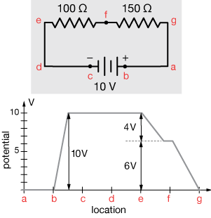
In this circuit, the 10 V battery creates a potential increase from points b to c. Part of that potential is "dropped" across the 100Ω resistor (4 V, according to Ohm's law, V = IR), and the other 6 V is dropped across the 150Ω resistor. Compare the circuit with the graph of voltage vs. circuit location.
Kirchoff's node or junction rule says that the total current into a node must equal the total current coming out of the node. The figure below shows the two kinds of scenarios we could encounter.

The node rule is a statement of the conservation of charge. Any charge coming into a node must leave by some route, and any charge leaving had to come from an incoming conductor.
Ohm's law relates current (I, in Amperes or "amps"), potential (voltage, V in Volts) and resistance (R in Ohms):
$$V = IR$$
Those are the tools we'll use to model these circuits.
Example 1
Consider the circuit below, containing several resistors and three current sources (batteries) arranged in two "loops," labeled
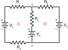
We can't work with this circuit in the same way that we did with previous circuits because these current loops aren't just branches of parallel elements. They each contain one or more of their own sources of current. We can, however still employ Ohm's law, V = IR, and Kirchoff's rules.
Notice that in the diagram above, junctions
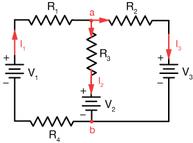
Now current I1 arrives at junction
$$I_1 = I_2 + I_3 \tag{1}$$
Then using Ohm's law and Kirchoff's loop rule on both loops, we have these equations:
$$ \begin{align} I_1 R_2 + I_2 R_3 + I_1 R_4 &= V_1 - V_2 \tag{2} \\[5pt] I_3 R_2 + I_2 R_3 &= -V_2 - V_3 \tag{3} \end{align}$$
In principle if we didn't know the three currents, we could find them using this information – one independent equation for each unknown. Now let's put some numbers on this circuit and see of we can do just that.
Here is the labeled circuit. For simplicity let's just make all of the resistances the same.
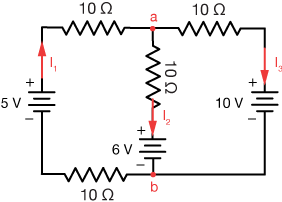
Now our equations (corresponding to equations 1, 2 and 3 above) are
$$ \begin{align} I_1 &= I_2 + I_3 \tag{1} \\[5pt] 10 I_1 + 10 I_2 + 10 I_1 &= 6 V - 5 V \tag{2} \\[5pt] 10 I_2 + 10 I_3 &= 10 V - 6 V \tag{3} \end{align}$$
These simplify to
$$ \begin{align} I_1 &= I_2 + I_3 \tag{1} \\[5pt] 20 I_1 + 10 I_2 &= 1 \tag{2} \\[5pt] 10 I_2 + 10 I_3 &= 4,\tag{3} \end{align}$$
where the units have been dropped for simplicity. Now we can take (3) and insert (1) like this:
$$ \begin{align} 10 I_2 + 10 I_3 &= 4,\tag{3} \\[5pt] 10 I_1 &= 4 \\[5pt] I_1 &= 0.4 \, A \end{align}$$
Now we can plug I1 into (2) to get $I_2 = -0.7 \, A.$ Notice that for I1 we got a positive current, confirming our initial "guess," and that for I2 we got a negative current. That indicates that the actual current flow is in the opposite direction of our original guess. Finally, I3 can be determined from equation (1):
$$ \begin{align} I_3 &= I_1 - I_2 \\[5pt] &= 0.4 - (-0.7) = 1.1 \, A \end{align}$$
Here's one more look at that circuit with the currents drawn in:
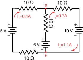
Take a minute to notice that Kirchoff's junction rule is obeyed for both junctions
Using matrices and inverse matrices to solve Example 1
There is another, more generally-useful way to solve three-equation systems like the one in example 1 that's worth going over here. You can do all of this on a TI-84 calculator, too.
Our sytem of three equations can be rewritten with the current variables in order, like this:
$$ \begin{align} I_1 - I_2 - I_3 &= 0 \tag{1} \\[5pt] 20 I_1 + 10 I_2 \phantom{0000} &= 1 \tag{2} \\[5pt] \phantom{0000} 10 I_2 + 10 I_3 &= 4 \tag{3} \end{align}$$
Now this can be expressed as a matrix-vector equation like this:
$$ \begin{bmatrix} 1 & -1 & -1 \\[5pt] 20 & 10 & 0 \\[5pt] 0 & 10 & 10 \end{bmatrix} \begin{bmatrix} I_1 \\[5pt] I_2 \\[5pt] I_3 \end{bmatrix} = \begin{bmatrix} 0 \\[5pt] 1 \\[5pt] 4 \end{bmatrix}$$
Now if we can express this matrix equation like this:
$${\bf M} \vec{I} = \vec{x},$$
where M is the 3×3 matrix, $\vec{I}$ is the vector of variables (what we're trying to find), and $\vec{x}$ is the column vector on the right side of the equal sign. Now such an equation can be solved using the inverse matrix of M, M-1, like this:
$$ \begin{align} {\bf M^{-1} M} \vec{I} &= {\bf M^{-1}}\vec{x} \\[5pt] {\bf I} \vec{I} &= {\bf M^{-1}}\vec{x} \\[5pt] \vec{I} &= {\bf M^{-1}}\vec{x} \end{align}$$
Given that ${\bf M^{-1} M} = {\bf I},$ where the matrix ${\bf I}$ is the identity matrix, and provided we can find the inverse matrix, we have our solution:
$$\vec{I} = {\bf M^{-1}} \vec{x}$$
The inverse matrix can be found by hand in simpler (e.g. 2×2 and 3×3) cases, but there are a number of handy computer algorithms for finding matrices and solving systems digitally. If you have a TI-84 or similar calculator, you can do it on that. The inverse matrix is
$$ {\bf M^{-1}} = \begin{bmatrix} 1 & 0 & 1/10 \\[5pt] -2 & 1/10 & -1/5 \\[5pt] 2 & -1/10 & 3/10 \end{bmatrix}$$
So our solution to these three equations is
$$ \begin{bmatrix} 1 & 0 & 1/10 \\[5pt] -2 & 1/10 & -1/5 \\[5pt] 2 & -1/10 & 3/10 \end{bmatrix} \begin{bmatrix} 0 \\[5pt] 1 \\[5pt] 4 \end{bmatrix} = \\[30pt] \begin{bmatrix} 1(0) + 0(1) + \frac{1}{10}(4) \\[5pt] -2(0) + \frac{1}{10}(1) - \frac{1}{5}(4) \\[5pt] 2(0) - \frac{1}{10}(1) + \frac{3}{10}(4) \end{bmatrix} = \begin{bmatrix} 0.4 \\[5pt] -0.7 \\[5pt] 1.1 \end{bmatrix}$$
These are just the solutions we found before.
Example 2
Calculate all of the currents in this circuit:
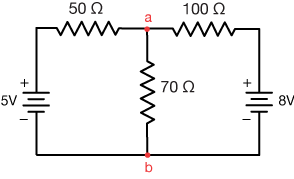
A look at the diagram shows that this is not just a circuit with parallel elements. It has two current loops, each with their own resistances and power supplies, so we'll have to solve some simultaneous equations to learn everything there is to know about it. In this example we'll solve this circuit in two ways to illustrate that you have choices in your approach. Here's one. We'll separate this circuit into the loops shown:
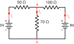
Choices for currents I1, I2 and I3 are already drawn in (red). Remember, the direction of current I1 is up to you, and currents I2 and I3 follow from it. We can then write three equations:
$$ \begin{align} I_1 &= I_2 + I_3 \tag{1} \\[5pt] 50 I_1 + 70 I_3 + 5 &= 0 \tag{2} \\[5pt] 100 I_2 - 8 - 70 I_3 &= 0 \tag{3} \end{align}$$
Notice that in the third equation, the $70 I_3$ term is negative because we're moving against our assigned I3 current. We're also sticking to conventional current through the batteries. We'll rearrange equations (1), (2) and (3) to
$$ \begin{align} I_1 - I_2 - I_3 &= 0 \tag{1} \\[5pt] 50 I_1 + 70 I_3 &= -5 \tag{2} \\[5pt] 100 I_2 - 70 I_3 &= 8 \tag{3} \end{align}$$
We can solve these three equations together in a number of ways; here's one. Let's use equation (1) to substitute $I_1 - I_2$ for I3 in (2) and (3).
$$ \begin{align} 50 I_1 + 70(I_1 - I_2) &= -5 \\[5pt] 100 I_2 - 70(I_1 - I_2) &= 8 \end{align}$$
Distributing the 70 in both equations gives:
$$ \begin{align} 120 I_1 - 70 I_2 &= -5 \\[5pt] -70 I_1 + 170 I_2 &= 8 \end{align}$$
We've eliminated I3 as a variable. Now multiply these equations by 17 and 7, respectively, to get ready to eliminate I2:
$$ \begin{align} 17(120 I_1 - 70 I_2) &= 17(-5) \\[5pt] 7(70 I_1 + 170 I_2) &= 7(8) \\ \hline \\[5pt] 2040 I_1 - 1190 I_2 &= -85 \tag{4} \\[5pt] -490 I_1 + 1190 I_2 &= 56 \tag{5} \end{align}$$
Adding the last equation (5) to (4) gives
$$ \begin{align} 1550 I_1 &= -29 \\[5pt] I_1 &= \frac{-29}{1550} = 0.0187 \, A \end{align}$$
From there it's simple to find
$$ \begin{align} I_3 &= 0.0581 \, A \: \: \text{and} \\[5pt] I_2 &= 0.0394 \, A \end{align}$$
Matrix method
We can also use the matrix method to solve these equations. Our three equations can be rewritten as
$$ \begin{align} I_1 - I_2 - I_3 &= 0 \\[5pt] 50 I_1 + 70 I_3 &= -5 \\[5pt] 100 I_2 - 70 I_3 &= 8 \end{align}$$
From there we obtain our matrix-vector equation:
$$ \begin{bmatrix} 1 & -1 & -1 \\[5pt] 50 & 0 & 70 \\[5pt] 0 & 100 & -70 \end{bmatrix} \begin{bmatrix} I_1 \\[5pt] I_2 \\[5pt] I_3 \end{bmatrix} = \begin{bmatrix} 0 \\[5pt] -5 \\[5pt] 8 \end{bmatrix}$$
The inverse of our matrix is
$$ {\bf M^{-1}} = \begin{bmatrix} \frac{14}{31} & \frac{17}{1550} & \frac{7}{1550} \\[5pt] \frac{-7}{31} & \frac{7}{1550} & \frac{6}{775} \\[5pt] \frac{-10}{31} & \frac{1}{155} & \frac{-1}{310} \end{bmatrix}$$
I calculated that matrix using a TI-84 calculator; more on that later. Multiplication of this inverse matrix by the (column) vector (0, 5, 8) gives the same soluions as we got above.
There's no unique choice of loops
In these two examples, we've chosen our loops as those that are side-by-side in the circuit, but really, all we need to find are three valid, independent equations that cover all of our circuit variables: currents, resistances and potential rises. Here is an equally valid way to solve this circuit using one of our previous loops and the full outer loop:
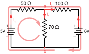
Let's solve this circuit just to show we get the same result. The relevant equations are:
$$ \begin{align} I_1 = I_2 &+ I_3 \tag{6} \\[5pt] 50 I_1 + 70 I_3 + 5 &= 0 \tag{7} \\[5pt] 50 I_1 + 100 I_2 - 8 + 5 &= 0 \tag{8} \end{align}$$
Rearranging these gives
$$ \begin{align} I_1 - I_2 - I_3 &= 0\tag{6} \\[5pt] 50 I_1 + 70 I_3 &= -5 \tag{7} \\[5pt] 50 I_1 + 100 I_2 &= 3 \tag{8} \end{align}$$
Now our matrix equation is
$$ \begin{bmatrix} 1 & -1 & -1 \\[5pt] 50 & 0 & 70 \\[5pt] 50 & 100 & 0 \end{bmatrix} \begin{bmatrix} I_1 \\[5pt] I_2 \\[5pt] I_3 \end{bmatrix} = \begin{bmatrix} 0 \\[5pt] -5 \\[5pt] 3 \end{bmatrix}$$
The inverse matrix is
$$ {\bf M^{-1}} = \begin{bmatrix} \frac{14}{31} & \frac{1}{155} & \frac{7}{1550} \\[5pt] \frac{-7}{31} & \frac{-1}{310} & \frac{6}{775} \\[5pt] \frac{-10}{31} & \frac{3}{310} & \frac{-1}{310} \end{bmatrix} \begin{bmatrix} 0 \\[5pt] -5 \\[5pt] 3 \end{bmatrix} = $$
$$ \begin{bmatrix} \frac{-5}{155} + \frac{3(7)}{1550} \\[5pt] \frac{5}{310} + \frac{3(6)}{775} \\[5pt] \frac{-15}{310} + \frac{3(-1)}{310} \end{bmatrix} = \begin{bmatrix} -0.0187 \\[5pt] 0.0394 \\[5pt] -0.0581 \end{bmatrix}$$
Again, these are the same currents as in our previous methods.
There is no unique choice of current loops when analyzing a multi-loop circuit. It's up to you. All that is necessary is to make sure that each resistor and voltage source is included at least once in one of the equations.
Example 3
Here is a three-loop circuit with three potential circuits. Currents I1 - I5 have been added to the diagram. Current I1 is first, and placed in an arbitrary direction. All of the other currents depend on that. The math will sort out the directions of the current, so long as we pay close attention to the orientations of the batteries. We'll assume that a positive current is the conventional (+ to - ) current.
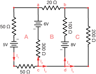
Loop A
$$ \begin{align} 50 I_1 + 50 I_1 + 300 I_2 + 5 + 6 &= 0 \\[5pt] 100 I_1 + 300 I_2 &= -11 \end{align}$$
Loop B
$$ \begin{align} 300 I_2 + 20 I_2 + 100 I_4 - 20 I_4 + 8 + 6 &= 0 \\[5pt] 320 I_2 + 80 I_4 &= -14 \end{align}$$
Notice that in loop B, we have two currents, I2 and I4 flowing to the top 20Ω resistor from opposite directions.
Loop C
$$ \begin{align} 100 I_4 + 200 I_5 + 8 &= 0 \\[5pt] 100 I_4 + 200 I_5 &= -8 \end{align}$$
Junction c
$$ \begin{align} I_1 &= I_2 + I_3 \\[5pt] I_1 - I_2 - I_3 &= 0 \end{align}$$
Junction d
$$ \begin{align} I_3 &= I_4 + I_5 \\[5pt] I_3 - I_4 - I_5 &= 0 \end{align}$$
Our matrix equation for this system of equations is
$$ \begin{bmatrix} 100 & 300 & 0 & 0 & 0 \\[5pt] 0 & 320 & 0 & 80 & 0 \\[5pt] 0 & 0 & 0 & 100 & 200 \\[5pt] 1 & -1 & -1 & 0 & 0 \\[5pt] 0 & 0 & 1 & -1 & -1 \end{bmatrix} \begin{bmatrix} I_1 \\[5pt] I_2 \\[5pt] I_3 \\[5pt] I_4 \\[5pt] I_5 \end{bmatrix} = \begin{bmatrix} -11 \\[5pt] -14 \\[5pt] -8 \\[5pt] 0 \\[5pt] 0 \end{bmatrix}$$
The inverse of the coefficient matrix is
$$ \begin{bmatrix} \frac{-1}{200} & \frac{3}{320} & \frac{3}{400} & \frac{3}{2} & \frac{3}{2} \\[5pt] \frac{1}{200} & \frac{-1}{320} & \frac{-1}{400} & \frac{-1}{2} & \frac{-1}{2} \\[5pt] \frac{-1}{100} & \frac{1}{80} & \frac{1}{100} & 1 & 2 \\[5pt] \frac{-1}{50} & \frac{1}{40} & \frac{1}{100} & 2 & 2 \\[5pt] \frac{1}{100} & \frac{-1}{80} & 0 & -1 & -1 \end{bmatrix}$$
Multiplying by the column vector $\vec{x} = (-11, -14, -8, 0, 0)$ gives these solutions:
$$ \begin{align} I_1 &= -0.1362 \, A \\[5pt] I_2 &= 0.0088 \, A \\[5pt] I_3 &= -0.1450 \, A \\[5pt] I_4 &= -0.2100 \, A \\[5pt] I_5 &= 0.0650 \, A \\[5pt] \end{align}$$
The negative currents indicate corrections in the initial current directions we chose to get started. Here's an updated picture of the circuit with the correct currents and directions:

Practice circuits
Solve for all voltage drops and currents everywhere in these DC circuits:
-
Problem here
Solution
Solution here
-
Problem here
Solution
Solution here
-
Problem here
Solution
Solution here
-
Problem here
Solution
Solution here
-
Problem here
Solution
Solution here
-
Problem here
Solution
Solution here
Conventional current
Conventional current is electric current that originates from the positive terminal of a power supply (battery) and moves toward the negative terminal. This direction was decided upon before early researchers knew that is electrons that move in circuits (electon current). It doesn't matter which current is used to solve for characteristics of most circuits, the same results will obtain.

![]()
xaktly.com by Dr. Jeff Cruzan is licensed under a Creative Commons Attribution-NonCommercial-ShareAlike 3.0 Unported License. © 2012-2025, Jeff Cruzan. All text and images on this website not specifically attributed to another source were created by me and I reserve all rights as to their use. Any opinions expressed on this website are entirely mine, and do not necessarily reflect the views of any of my employers. Please feel free to send any questions or comments to jeff.cruzan@verizon.net.