Sampling a population
In statistical analysis, we're usually trying to find out something about a population by surveying or querying a small sample (a simple random sample, or SRS) of that population.
For example, we might like to know how the U.S. population of eligible voters (about 240 million people) will vote – say either for the Democrat or for the Republican – in the next election. It wouldn't be practical to survey all 240 million people (or even a million), and at any rate, doing so would be called an election! Instead, we choose a smaller group randomly from the population and ask how those people will vote. If we're careful, the results of that sample will be a faithful estimate of the characteristic of the population we're trying to measure.
When we perform such a measurement, we're generally estimating a proportion (what fraction of the voters will select the Democrat?) or a mean (like what is the average height of all American women over 20 years of age?). Proportions and means will be recurring themes for us as we go on.
The properties that characterize a population are called parameters. We generally reserve the letters $p$ (for proportion) and $\mu$ (for the mean) when referring to populations.
We make carefully-designed random samples of populations which are small enough that we can calculate proportions or means that we'll use to estimate population parameters. These proportions $( \hat p \;$ pronounced "p hat"$)$ and means $( \bar x)$ are called statistics.
mnemonic
Population → Parameter
Sample → Statistic
Statistics always estimate parameters.
There is a table of definitions relative to sampling at the bottom of this page.

About sample size & quality
This subject can be a little tricky for students who have learned advanced algebra and calculus because it has "fuzzy edges." In other math disciplines, there is a right and a wrong answer, and if we want more precision in an answer, we can just calculate it. In statistics, the mathematics of uncertainty, we have to do a little more educated guessing, but we try to back it up with solid reasoning. Here we go.
Number of individuals: $n$ of $N$
When we're taking samples from a population of $N$ individuals, it's usually done without replacement. Recall that if we draw a face card from a 52-card deck, which originally contained 12 face cards, the chance of drawing another face card changes from the original $\frac{12}{52} = 0.2307$ to $\frac{11}{51} = 0.2156$, a significant difference (about 6.5%), so drawing each member of a sample is not independent of the other draws. But we simply can't practically draw samples from a large populations with replacement, so we need some compromise, and this is it:
The number of individuals sampled from a population should be fewer than 10% of the population.
That is, $n \le \frac{1}{10}N$ or $N \ge 10 n$, where $N$ is the number of individuals in the population and $n$ is the number in each sample.
This rule of thumb turns out, on average, to preserve just enough of the independence of random sample selection for the statistics we derive from our samples to be meaningful. It's not a hard science, just something that's been tested and agree-upon for a long time. You should also be aware that in certain fields, a different standard might apply; it depends on the context.
Sample size, $n$
A general rule of thumb in statistics is that sample size — the number of individuals from a population included in a sample — should be 30 or more. There's a lot rolled up in that, and it's not always true (in fact it's a matter of some debate in some fields), but we'll stick with it for now.
Sample size should be $n \ge 30$
Proportions: Large count conditions
When we're working with sample proportions (instead of means), getting a representative sample depends on the proportion. Let's take an example: A jar filled with a large number of jelly beans (let's say 1000), half red, half black, so $p = 0.5$. It's easy to see that in choosing a sample of 100 beans (10% of the total), we will choose samples with, on average, the same proportion, $\hat p = 0.5$.
Now imagine that the proportion is $p = 0.05$, or 5% of the beans are red. Now in taking samples of size $n = 100$, it's conceivable that we could come up with a large number of such samples with far less than 5% red beans. That is, it would be likely that our distribution of sample proportions would be skewed to the black side.
In order to get around this issue, we make another rule of thumb (two, actually), called the large-count conditions. They are:
$$ \begin{align} n p &\gt 10 \\[5pt] n (1 - p) &\gt 10, \end{align}$$
where $n$ is the number of individuals per sample and $p$ is the population proportion, often approximated by the sample proportion, $\hat p$. Now $np$ and $n(1-p)$ cover the minority populations on both ends of the proportion spectrum, so checking that both of these are at least 10 is some assurance of a non-skewed distribution. We saw the large-count conditions when we approximated a binomial distribution with a normal distribution.
Let's look at our jelly-bean example, and assume that $p = 0.05$. We have
$$ \begin{align} n p &\gt 10 \; \longrightarrow \; 100(0.05) = 5 \\[5pt] n (1 - p) &\gt 10 \; \longrightarrow \; 100(1-0.05) = 95 \end{align}$$
So this scenario passes if we look at it from the point of view of the black beans, which constitute 95% of the sample: Any sample is likely to have something like 95% black beans. But on the other point of view, $np \lt 10$, means that we'd probably be able to make a large number of samples with well below 5% red beans, thus misrepresenting that proportion.
It's important to realize that this is a rule of thumb, not a something rigorously proved from the mathematics. In fact, in older textbooks the number 10 was 5, and many modern statisticians would insist on something more like 15. It's also a bit case-dependent, so in a real problem doing some simulations and making some graphs in order to validate the methods used would be prudent.
Finally, the large-count conditions for sample size apply only to sample proportions. Here's a basic flowchart for constructing samples:

The Means and proportions of samples
Imagine for a minute that you could take every possible sample of size 10 from a population of 100, given that the mean of the population was $\mu ± \sigma$. Would the sample mean, $\bar x$, equal $\mu$? Don't sweat the details of the math just now – we'll cover it later and it's easy – but if we think about it, the number of possible sets of 10 that can be taken from a set of 100 is the binomial coefficient
$$ \require{cancel} \begin{align} \binom{100}{10} &= \frac{100!}{10!(100-10)!} \\[5pt] &= \frac{100 \cdot 99 \cdot \dots \cdot 91 \cdot \cancel{90!}}{10!(\cancel{90!})} \\[5pt] &\approx 1.73 \times 10^{13} \; \text{samples} \end{align}$$
That's an enormous number of samples, and it clearly oversamples the data set of 100, so we'd expect, without giving a proof here, that the mean of samples (the mean of the sampling distribution) would equal the population mean, $\mu$.
We say that the mean of the sampling distribution, $\bar x$, is an unbiased estimator of the population mean, because if we have enough samples, the mean of the sampling distribution will tend toward $\mu$.
Unbiased estimators
For sample means, the mean of the sampling distribution $\bar x$ is an unbiased estimator of the population mean $\mu$.
For sample proportions, the mean of the sampling distribution $\mu_{\hat p}$ is an unbiased estimator of the population proportion $p$.
Here's an example so you can see how this works.
Example 1
As an example of a complete sampling distribution, let's take the set $\{1,2,3,4,5,6,7\}$ and enumerate all possible samples of size two, then calculate the mean and standard deviation.
First, the mean is clearly 4, and the standard deviation (you'd have to calculate it) is 2. Here are the possible samples and their means:
| S | $\bar x$ | S | $\bar x$ |
|---|---|---|---|
| {1,2} | 1.5 | {2,7} | 4.5 |
| {1,3} | 2.0 | {3,4} | 3.5 |
| {1,4} | 2.5 | {3,5} | 4.0 |
| {1,5} | 3.0 | {3,6} | 4.5 |
| {1,6} | 3.5 | {3,7} | 5.0 |
| {1,7} | 4.0 | {4,5} | 4.5 |
| {2,3} | 2.5 | {4,6} | 5.0 |
| {2,4} | 3.0 | {4,7} | 5.5 |
| {2,5} | 3.5 | {5,6} | 5.5 |
| {2,6} | 4.0 | {5,7} | 6.0 |
| {6,7} | 6.5 |
There are
$$ \require{cancel} \begin{align} N &= \binom{7}{2} = \frac{7!}{2!(7-2)!} \\[5pt] &= \frac{7 \cdot 6 \cdot \cancel{5!}}{2 \cdot \cancel{5!}} \\[5pt] &= \frac{42}{2} = 21 \end{align}$$
possible groups of two from this group of seven; all are shown in the table.
If we take the mean of this sampling distribution – the mean of the sample means shown in the table, we get $\bar x = 4$, precisely the mean we calculated above. Here's a dotplot of the entire sampling distribution.

This is always the case for sampling means that include all possible combinations, with the benefit that the sampling distribution always tends toward a normal distribution, no matter what the underlying population distribution.
Just to show that the dotplot distribution is indeed normal, here's a plot of the data vs. the expectations for a standard-normal distribution (Z-scores at each percentile). The points fall on a line, so the distribution is normal.

Sample proportions
If our population is characterized by some proportion $p$ (a parameter), then taking several samples from a population, each with proportion $\hat p$, will produce a mean of proportions, $\mu_{\hat p}$. A proportion might be something like
- proportion of registered voters who are Independents
- proportion of jelly beans that are green
- proportion of U.S. counties with over 100,000 people
A proportion differs from a mean in that we don't immediately think of calculating an average from a single sample. When we ask a sample of people whether they like chocolate or vanilla ice cream better, we simply count the results and take a ratio. Nothing is averaged.

If we take $N$ randomly-chosen samples from the population, we expect that, while the sample proportion $\hat p$ can vary, a distribution of them – the sampling distribution of proportions – will have a mean that predicts the population parameter, $p$. Thus, $\hat p$ is an unbiased estimator of $p$.
If we choose a number of individuals per sample $(n)$ that is less than or equal to 10% of the population, and if we ensure that the large-count conditions apply:
$$np \ge 10 \phantom{000} \text{and} \phantom{000} n(1-p) \ge 10,$$
then we have
$$\hat p = p$$
and the standard deviation is
$$\sigma_{\hat p} = \sqrt{\frac{p (1 - p)}{n}}$$
Notice that the standard deviation of the sample means decreases as the square root of the number of samples, $n$.

Sample proportions
The mean of a distribution of sample proportions (the sampling distribution) approaches the population proportion, $p$.
$$\hat p = p$$
The standard deviation of a sampling proportion is
$$\sigma_{\hat p} = \sqrt{\frac{p (1 - p)}{n}}$$
The standard deviation decreases as the square root of the number of samples. Sometimes this is written as
$$\sigma_{\hat p} = \sqrt{\frac{pq}{n}},$$
where $q = 1 - p$. It's just an alternate notation that's a little neater.
Example 2
Imagine that 42% of voters in a city are in favor of a particular ballot question. A sample of 500 voters is randomly selected and asked if they favor the question.
- Determine whether this sample and situation meets the conditions to consider the sampling distribution to be approximately normal (and thus be able to use the familiar tools of a normal distribution).
- Calculate the probability that the sample proportion will be within ±5% of the true population proportion.
$$ \begin{align} np &= 500 (0.42) = 210 \gt 10 \\[5pt] n(1-p) &= 500(0.58) = 290 \gt 10. \end{align}$$
So the sampling distribution should be normal and we can continue using the tools of the normal distribution.
For (b), we can set the sample mean $\hat p$ to the population mean, $\hat p = p = 0.42$. Then the standard deviation of the sample is
$$ \begin{align} \sigma_{\hat p} &= \sqrt{\frac{p(1-p))}{n}} \\[5pt] &= \sqrt{\frac{0.42(0.58)}{500}} \\[5pt] &= 0.0221 \end{align}$$
Now we want to know the probability that a sample mean will lie between 0.42-0.05 and 0.42+0.05, or in the interval [0.37, 0.47]. The relevant Z-scores are
$$ \begin{align} Z_{0.37} &= \frac{0.37 - 0.42}{0.0221} = -2.2624\\[5pt] Z_{0.47} &= \frac{0.47 - 0.42}{0.0221} = \, 2.2624 \end{align}$$
Then we can use normalcdf( ) on a TI-84 calculator,
normalcdf(-2.2624, 2.2624, 0, 1) = 0.9764
Interpretation: We would expect about 97% of samples of 500 voters to have proportions between 37% and 47%.
The normalcdf( ) function can be used more directly, too, by simply entering the mean and standard deviation of the sample without Z-score conversion:
normalcdf(0.37, 0.47, 0.42, 0.0221) = 0.9764
You can (should) check that for yourself.
Example 3
A retailer claims that 90% of all their orders are shipped within 24 hours of being received. A consumer-advocacy group tested the retailer by placing 110 orders of different merchandise at different times of day and week, selected randomly. 98 of the orders were shipped within 12 hours.
- Confirm that the sample size and quality are enough to assume that the sample proportion takes a normal distribution.
- Assuming that the retailer's claim was true, calculate the probability that 98 of 120 orders or fewer would ship on time. What can you conclude about the retailer's claim?
$$ \begin{align} np &= 110(0.9) = 99 \gt 10 \\[5pt] n(1-p) &= 110(0.1) = 11 \gt 10 \end{align}$$
The sample proportion is $\hat p = p = 0.9$, and the standard deviation is
$$ \begin{align} \sigma_{\hat p} &= \sqrt{\frac{p(1-p)}{n}} \\[5pt] &= \sqrt{\frac{0.9(0.1)}{110}} \\[5pt] &= 0.0286 \end{align}$$
The Z-score for 98 of 110 on-time orders (0.8909) is
$$Z = \frac{0.89-0.90}{0.0268} = -0.3496$$
Using a TI-84 calculator, we find
normalcdf(-1E99, -0.3496, 0, 1) = 0.3633
So there's about a 36% chance that even fewer orders could be shipped to still comply with the retailer's claim. It's a valid claim.
Sample means
Now let's consider the other kind of sampling distribution problem, distributions of sample means. When we take a sample that measures some parameter with units, such that we'd be inclined to take an average, that's what we're talking about. Some examples could be
- Average MCAT® scores for a year,
- Average weights of newborns in a county,
- Average price of regular gasoline in a large city.
As a reminder, we require that the number of individuals sampled be less than or equal to the population number, $N \le 10n$, and that the number of individuals in the sample be at least 30, $n \ge 30$. If these conditions are met, then the sampling distribution of means approaches a normal distribution, and whatever th shape of the distribution of the population, we can still employ our normal distribution tools to solve problems.
Here's a picture of how it works.

The distribution of sample means ($\bar x$, means of individual samples) tends toward being normally distributed, so we say that $\bar x$ is an unbiased estimator of the population mean $\mu$, a parameter.
Then the standard deviation of a sample is inversely proportional to the square root of the number of individuals in the sample:
$$\sigma_{\bar x} = \frac{\sigma}{\sqrt{n}}$$
where $\sigma$ is the population standard deviation. That version of $\sigma$ is actually called the standard error.
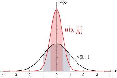
The graph below illustrates the difference between a population and its mean and standard deviation (illustrated by the black curve, a normal distribution with mean $\mu = 0$ and $\sigma = 1$ — the standard normal distribution (SND), actually. Superimposed on it is the distribution $N(\mu, 1/\sqrt{5})$, to which our SND would change upon averaging five sample means.
Notice that the larger denominator gives us a narrower distribution. The areas of the red and gray-shaded regions are 68% of the total probability, or $\mu - \sigma \lt P \lt \mu + \sigma$.
For sample means, we only require that two conditions be met for the sample size. They are
$$ \begin{align} n &\ge 30 \\[5pt] n &\le \frac{N}{10}, \end{align}$$
where $N$ is the population size. Now let's do a couple of examples to see how this all works.
Sample means
The mean of a distribution of sample means (the sampling distribution) approaches the population mean, $\mu$.
$$\bar x = \mu$$
The standard deviation of a sample mean is
$$\sigma_{\bar x} = \frac{\sigma}{\sqrt{n}}$$
The standard deviation decreases inversely as the square root of the number of samples.
The adjusted standard deviation is called the standard error.
Example 4
The recognized average time it takes for a human to react to a visual stimulus is 0.25 seconds with a standard deviation of about 20 ms (0.020 s). Suppose we performed a sample of 100 people and obtained a sample mean reaction time of 0.23 seconds. Would we conclude that there's something special about this population?
We expect that $\bar x = \mu = 0.25$ and that the standard error in this case will be
$$ \begin{align} \sigma_{\bar x} &= \frac{\sigma}{\sqrt{n}} \\[5pt] &= \frac{0.020}{\sqrt{100}} \\[5pt] &= 0.002 \end{align}$$
So for this sample, $\bar x ± \sigma_{\bar x} = 0.25 ± 0.002 \, \text{seconds}$.
Now let's evaluate whether a reaction time of 0.21s would be surprising. We can do it two ways. First, the Z-score would be
$$Z = \frac{0.23 - 0.25}{0.002} = \frac{-0.02}{0.002} = -10$$
We don't really need to calculate the probability of a reaction time equal to or less than 0.023 s because our Z score shows that this is more than ten standard deviations away from the mean. Just for drill, though, we can use a TI-84 calculator to find the probability:
normalcdf(-1E99, -10.0, 0, 1) = 0
Likewise, we could use normalcdf( ) directly like this:
normalcdf(-1E99, 0.23, 0.25, 0.002) = 0
We'd have to conclude that we wouldn't likely arrive at this reaction time from a sample of 100 people by random chance, so there must be something to it. This must be a special group.
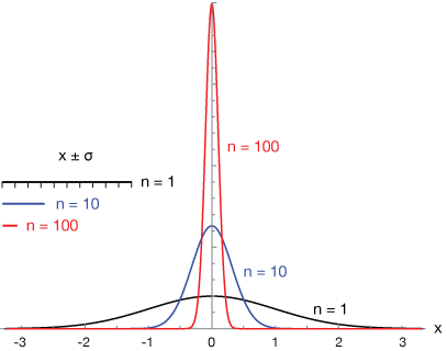
Pro tip
The standard deviation of a mean of samples gets smaller with the number of means or proportions sampled. But it doesn't get linearly smaller (it's not directly proportional). We say that the standard deviation "goes as" 1 over the root of the number of trials. That means that if we want the standard deviation to be 10 times smaller, we'll have to sample 100 means or proportions. The graph shows a normal distribution with one sample (black), 10 samples (blue) and 100 samples (
Example 5
The length of time (hours) of an average high school soccer game is 1.75 h with a standard deviation of 0.21 hours. Suppose that a sample of 25 games is taken.
- Is the distribution of sample means normal?
- Calculate the mean and standard deviation of the sample means.
- Calculate the probability that the mean of the sample is less than 1.7 hours.
- Calculate the probability that the mean of the sample is more than 2 hours.
The mean of the sample should be $\bar x = \mu = 1.75$. The standard deviation for 25 samples is
$$\sigma_{\bar x} = \frac{0.21}{\sqrt{25}} = 0.0420$$.
Now the probability that the average length of a game out of 25 samples will be less than 1.7 hours can be calculated by calculating the Z-score,
$$Z = \frac{1.7 - 1.75}{0.0420} = -1.1905$$
Then using normalcdf( ) on a TI-84, we get
normalcdf(-1E99, -1.19, 0, 1) = 0.1170
So there's about a 12% chance of a game lasting 1.7 hours or less time.
For (d), we have
$$Z = \frac{2 - 1.75}{0.0420} = 5.9524$$
We don't really need to do a calculation here because that's about six standard deviations from the mean. It would be very unlikely for a game to last 2 hours or longer. There's no need to quibble about the details.
| Term | Definition | Symbol |
|---|---|---|
| Parameter | Describes a feature of a population, like a mean of a measurement or a proportion of the population. | |
| Statistic | Describes a feature of a sample, an analog to a parameter; Statistics estimate parameters. | |
| Population mean | Mean value of a measurement of an entire population, often not known or even knowable | $\mu$ |
| Population proportion | Proportion of a population with some characteristic, such as food choice, often not known or even knowable | $p$ |
| Sample mean | Mean value of a measurement of a sample of a population | $\bar x$ |
| Sample proportion | Proportion of a sample with some characteristic | $\hat p$ |
| Number of samples | Number of samples in a sampling distribution or Number of individuals in a population |
$N$ |
| Number of individuals | Number of individuals in each sample (usually the same across all samples) | $n$ |
| Sample size | $N \gt 10 n$ or $n \le \frac{N}{10}$ | |
| Sample size minimum | $N \gt 30$ | |
| Large-count conditions | $np \gt 10$ and $n(1 - p) \gt 10$ |
Simulation
Here is an interactive simulation of building a sampling distribution from an underlying distribution that is not Normal. The underlying distribution is the uniform distribution of numbers between 1 and 100, each with equal probability of occuring:
$$ \begin{align} P(1) &= P(2) = \dots = P(100) = \frac{1}{100} \\[5pt] \text{or } \; P(X_i) &= \frac{1}{100} \end{align}$$
You can see that the mean of the sampling distribution is pretty consistently about half way through the distribution, about $X = 50$, and the distribution appears to be roughly Normal. We'll see below that if we take enough sample from any non-Normal distribution, the resulting sampling distribution will tend toward a Normal distribution.
The Central Limit Theorem is the basis of why we can do many of the statistical analyses we do. In brief, it says that no matter what the population distribution looks like, if we take enough samples (provided they meet all of our conditions), the distribution of the sample means or sample proportions (the sampling distribution) will be approximately normal, and will actually tend more and more toward normal as we add samples.
It might be useful to use an extreme example. Let's first construct an odd distribution like an exponential decay. It might look like this:

This is clearly not a normal distribution. We've chosen the function $f(x) = e^{-0.25x}$. Now we'll take 1000 samples using x-values from 1 to 10 and distribute them accordingly:

The mean and standard deviation are $3.62 ± 2.48$, as calculated from the table of values and probabilities of this discrete random variable below.
![]()
Now let's generate a bunch of random samples of 100 values from this distribution. I used a little Python program to do that. It's basically an array of 241 1's, 188 2's, and so on, then random samples of some size are drawn from that – with replacement. Normally we'd choose our samples without replacement, but the error will be small in this case, and we'll still be able to prove our point.
Here is a histogram of the results of averaging samples of 30 draws from our distribution. 100 such samples were made. Both a normal distribution (gray curve) and our exponential decay (red curve) are sketched on the histogram. We can see that the distribution has some of the characteristics of both. It's not a great looking normal curve and it still looks a little like an exponential decay.

Here's what happens when we take 100 samples of 100 individual members of the population. Now the curve looks a lot more normal in shape, and the average of the samples is 3.60, very close to the population mean.

We can't add any more individuals to these samples because they're already at the 10% limit (though our replacement scheme really takes care of that here), but we can average a few more samples. This histogram shows the result of plotting 200 samples of 100 individuals each. It looks even better (more of a normal curve), and the mean is right on our population value of 3.63.

This little example is not a proof of the Central Limit Theorem, but it's a convincing example. Despite a population distribution that was anything but normal, when we took a number of well-constructed random samples and plotted its distribution, it got closer to normal in form and better at reproducing the population mean as our sample size and number of samples increased.
Central Limit Theorem
If enough samples are taken from any population distribution, even if it is not normal, the distribution of sample means or proportions will tend toward normal as we increase the sizes and number of those samples.
The advantage that this gives us is that we can use the tools we've learned from normally-distributed data to analyze nearly any data set, so long as our sampling is well-constructed.
Simulation-2
In this simulation, we'll randomly select points from the distribution below, a decaying exponential distribution,
$$P(X) = \frac{1}{2} e^{\frac{-x}{2}}$$
This is a normalized distribution (total area under the curve = 1), and is clearly nothing like a Normal distribution.

We'll take random samples of ten from this distribution, average the ten $X$ vlaues and plot each average as a point on the dot plot. The simulation will show that if we take enough samples of 10, the distribution of those sample averages will approach a normal distribution. This is an example of the central limit theorem, explained below.
Click to see calculation of the mean of this distribution (calculus).
The mean value of a probability distribution with random variable $x$ is
$$E(x) = \int_{-\infty}^{\infty} x P(x) \, dx$$
where $P(x)$ is the probability distribution of $x$. Because this distribution isn't defined for $x \lt 0$, we need to solve this improper integral:
$$E(x) = \frac{1}{2} \int_0^{\infty} x e^{-x/2} \, dx$$
We can do this integral by parts starting like this:
$$ \begin{align} u &= x, \phantom{000} dv = e^{-x/2} dx \\ du &= dx, \phantom{000} v = -2 e^{-x/2} + C \end{align}$$
Then we can put our integral together, solve it and do the substitutions:
$$ \begin{align} \frac{1}{2}\int_0^{\infty} &x e^{-x/2} \, dx \\[5pt] &= \frac{1}{2} \bigg[ -2 x e^{-x/2} + 2 \int e^{-x/2} \, dx \bigg] \\[5pt] &= \frac{1}{2} \bigg[ -2xe^{-x/2} - 4e^{-x/2} \bigg]\bigg|_0^{\infty} \\[5pt] &= \frac{1}{2} \bigg[ -(2x + 4) e^{-x/2} \bigg] \bigg|_0^{\infty} \\[5pt] &= \frac{1}{2} \bigg[ \lim_{x \to \infty} \frac{-(2x+4)}{e^{-x/2}} - \lim_{x \to 0} \frac{-(2x+4)}{e^{-x/2}} \bigg] \\[5pt] &= \frac{1}{2} [0+4] = 2 \end{align}$$
The average value of the distribution is $x = 2$.
Click for details about the simulation.
How the simulation was done
There are a few ways to simulate selection of random samples from a defined distribution like the one modeled in this simulation,
$$P(X) = \frac{1}{2} e^{-x/2}.$$
Two of those are
- The inverse CDF method, and
- The Monte Carlo method.
Here's the idea behind the first. The function $P(X)$ is the probability function. Put in a value of X and it will give you the probability of the occcurence of that value in the distribution. In our sample distribution here, small values of $X$ are more probable than larger ones. The distribution is shown in the red curve in the graph below. It's a normalized probability function, by the way, meaning that the total area under the curve from $x=0$ to $\infty$ is one.

What we're interested in is the cumulative distribution function (CDF), a function that gives the area under $P(X)$ from left to right. That function is obtained by doing the integral
$$\text{CDF}(X) = \frac{1}{2} \int_0^x e^{-t/2} \, dt$$
where $t$ is a dummy variable in this integral-defined function. Here's the integral:
$$ \begin{align} \text{Let } u &= -X/2, \text{ then } dX = -\frac{1}{2} dX \\[5pt] - \int_0^{-X/2} e^u \, du &= -[e^u] \big|_0^{-X/2} \\[5pt] &= -[e^{-X/2} - 1] \\[5pt] \text{CDF}(X)&= 1 - e^{-X/2} \end{align}$$
The CDF function is drawn in black in the graph above. Notice that it has a horizontal asymptote (dashed line) at $y = 1$. That makes sense because it represents the area under the $P(X)$ curve. The amount of area gets smaller as $x$ gets larger, so we add increasingly less area to the growing sum. It's limit is 1 because this is a normalized PDF
The graph below shows how our CDF works. Area is added or integrated from left to right. Here we've added up all of the area under the curve between $X = 0$ and $X = 4$. It means that there is an 86.5% chance of randomly selecting an $X$ value between 0 and 4 from this distribution.

Random selections from the distribution
In order to select randomly from this distribution, we'll use the inverse of the CDF. First, here's how that is obtained.
Solve for $Y$ to get the inverse function, $\text{CDF}^{-1}$:
$$ \begin{align} Y &= 1 - e^{-X/2} \\[5pt] Y - 1 &= -e^{-X/2} \\[5pt] 1 - Y &= e^{-X/2} \\[5pt] ln(1 - Y) &= -\frac{X}{2} \\[5pt] -2 ln(1 - Y) &= X, \; \text{ so} \\[5pt] \text{CDF}^{-1} &= -2 ln(1-Y) \end{align}$$
Now this inverse function will give us a location, $X$, in the domain of the CDF for every Y value we randomly generate. What remains is to generate random numbers between 0 and 1 (the range of the CDF) and use $\text{CDF}^{-1} to calculate the corresponding value from the domain, then plot that value on the dot plot.
Monte Carlo method
The Monte Carlo method is based on random chance. The idea is illustrated in the graph. We simply choose a random (X, Y) pair from the domain and range of our probability function, $P(X)$, and test it to see if it's on our below our function. If it is, we keep it. If not, we move on to the next point. In that way we can collect samples of any size from under our function.

Practice
-
The average U.S. Marine does 300 ± 50 push ups per day (50 = one standard deviation). Let's say we take a random sample of 40 Marines. What is the probability that the sample mean is at most 320 push ups per day?
Solution
The population mean and standard deviation are given:
$$\mu ± \sigma = 300 ± 40$$
Our statistics will be $\bar x ± \sigma_x$. The mean is an unbiased estimator of the population mean, $\mu$, so $\bar x = 300$. For the standard deviation, we have
$$ \begin{align} \sigma_x &= \frac{\sigma}{\sqrt{n}} \\[5pt] &= \frac{50}{\sqrt{40}} = 7.9 \end{align}$$
where $n = 40$ is the sample size.
So our sample statistics are $\bar x ± \sigma_x = 300 ± 8$ (rounded to the nearest push up).
The expression
$$\frac{\sigma}{\sqrt{n}}$$
is called the standard error.
-
The distribution of incomes in a certain town are right-skewed with a mean of \$37,000 and a standard deviation of \$6,000. A random sample of 60 households is taken.
- Calculate the sample mean and its standard deviation.
- Calculate the probability that the sample mean is greater than \$38,500.
Solution
The sample mean is $\bar x = 37,000$ (because the sample mean (a statistic) is an unbiased estimator of the population mean (a parameter). The standard error is
$$\sigma_{\bar x} = \frac{\sigma}{\sqrt{n}} = \frac{6,000}{\sqrt{60}} = 774.5967$$
For (b) the Z score is
$$Z = \frac{38,500 - 37,000}{774.5967} = 1.9365$$
We can use a standard normal table or a TI-84 calculator to find the solution:
normalcdf(1.9365, 1E99, 0, 1) = 0.0264
So there's a 2.6% chance of observing an average income of \$38,500 or above in a sample of 60 incomes.
-
The teacher's salaries in an independent school (typically, independent school teacher salaries are lower than those of a public school) have a mean of \$55,000 ± \$5,200. Suppose we take a sample of 25 teachers from the school.
- Calculate the probability that the sample mean salary will be greater than \$54,000.
- Calculate the probability that the sample mean salary will be less than \$49,000.
- Calculate the probability that the sample mean salary will be between \$52,000 and \$55,000.
Solution
(a) The sample mean is $\bar x = 55,000$ and the sample standard deviation (standard error) is
$$\sigma_x = \frac{5,200}{\sqrt{60}} = 671$$
Now for a sample size of 60, we can safely assume that the sampling distribution will be approximately normal, thus we can calculate a Z-score,
$$Z = \frac{54,000 - 55,000}{671} = -1.4903$$
Now we can use the normalcdf() function on a TI-84 calculator to find the appropriate area under the standard normal distribution:
normalcdf(-1.4903, 1E99, 0, 1) = 0.9319
So the probability of a salary over \$54,000 at this school is about 93%.
(b) We approach this one the same way, by starting with the Z-score, which maps our problem onto the standard normal distribution.
$$Z = \frac{49,000 - 55,000}{671} = -8.9419$$
Already, with that kind of Z-score, we'd expect this probability to be small, but let's calculated on a TI-84:
normalcdf(-1E99, -8.9419, 0, 1) = 0.0000
Indeed, to four decimal places, the probability is zero.
(c) The Z-scores for these two salaries are
$$ \begin{align} Z_1 &= \frac{52,000 - 55,000}{671} = -4.4709 \\[5pt] Z_2 &= \frac{55,000 - 55,000}{671} = 0 \end{align}$$
Then the area under the standard normal curve is
normalcdf(-14.4709, 0, 0, 1) = 0.5000
That means that half of the salaries are between these two.
-
The pollen count distribution for a city in a certain month is not normally distributed, with $\mu = 8.0$ and $\sigma = 1.0$. A sample of 64 measurements is taken. Calculate the 75th percentile of the sample mean.
Solution
We have the sample parameters $\mu = 8.0 ± 1.0$, and there are 64 measurements in the sample, so we can expect the sampling distribution to be approximately normal, according to the central limit theorem. The 75th percentile is the location in the distribution at which is above 75% of the total probability. We can use a table of values or a TI-84 calculator to find the Z-score that goes with an area of 0.75:
invNorm(0.75, 0, 1) = 0.6745
Now the Z-score definition is
$$Z = \frac{X - \mu}{\sigma},$$
We'll need to use the standard error instead of the population standard deviation. That's
$$\sigma_X = \frac{\sigma}{\sqrt{n}} = \frac{1.0}{\sqrt{64}} = 0.125$$
Then we can use the Z-score to solve for the value of X (pollen count) at the 75th percentile:
$$ \begin{align} Z \sigma &= X - \mu \\[5pt] X &= Z \sigma + \mu \\[5pt] X &= 0.6745(0.6745) + 8.0 \\[5pt] &= 8.08 \approx 8.1 \end{align}$$
A pollen count at X = 8.1 would be at the 75th percentile of measurements for this region.
-
In 2019, according to the U.S. Department of Energy (DOE), the average car occupancy in the U.S. was 1.5 persons per vehicle. The standard deviation of that study wasn't cited, but let's assume it's $\sigma = 0.05$. Suppose we observe 50 cars in a large city and count the occupants, arriving at a mean of 1.52. Might we conclude that this city is really different from the U.S. average in this regard?
Solution
The population mean is $\mu ± \sigma = 1.5 ± 0.05$. Then we have the sample mean of $\bar x = 1.5$ and sample standard deviation
$$\sigma_x = \frac{\sigma}{\sqrt{n}} = \frac{0.05}{\sqrt{50}} = 0.0071$$
Now the Z-score for a mean of 1.52 is
$$Z = \frac{1.52 - 1.5}{0.0071} = 2.8169$$
Now we can use a TI-84 calculator to find the likelihood of a mean greater than 1.52. It is
normalcdf(2.8169, 1E99, 0, 1) = 0.0024
There is a 0.24% chance of a mean larger than 1.52, so we'd consider a mean of 1.52 to be rare, and conclude that this city could indeed be a different type of city in this regard.
-
Newborn American Bison have an average weight of 32.5 ± 5 pounds (5 lb. is one standard deviation). What is the probability that in a study of 30 newborn bison, the mean weight is less than 30.0 lbs.?
Solution
The sampling mean and standard deviation are
$$ \begin{align} \bar x &= 32.5 \\[5pt] \sigma_{\bar x} &= \frac{\sigma}{\sqrt{n}} = \frac{5}{\sqrt{30}} \\[5pt] &= 0.9128 \end{align}$$
The Z-score in this distribution for a weight of 31 lbs. is
$$Z = \frac{x - \bar x}{\sigma_{\bar x}} = \frac{31 - 32.5}{0.9128} = -1.6433$$
Now using a calculator to calculate the area from the extreme left of the distribution to Z = -1.6433, we get
normalcdf(-1E99, -1.6433, 0, 1) = 0.0502
The probability of finding an average weight this low is about 5%, so if that measurement did obtain, it would be worth further exploration.

![]()
xaktly.com by Dr. Jeff Cruzan is licensed under a Creative Commons Attribution-NonCommercial-ShareAlike 3.0 Unported License. © 2012-2025, Jeff Cruzan. All text and images on this website not specifically attributed to another source were created by me and I reserve all rights as to their use. Any opinions expressed on this website are entirely mine, and do not necessarily reflect the views of any of my employers. Please feel free to send any questions or comments to jeff.cruzan@verizon.net.